6 Styling tables
We can use R to build tables programmatically so that labelling, formatting and styling are completely reproducible. We will show the steps involved in creating a publication-ready table using the gt package. The syntax is relatively straightforward and the results can be outputted to Word and PDF.
6.1 gt tables
Before formatting and styling the table it is a good idea to understand the structure and syntax of a gt table. This is important because the functions in the gt package are named so that they relate to the parts of the table.
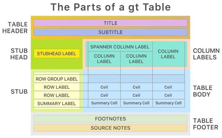
- Table header: title and subtitle
- Stub and Stub Head: area to left of table containing row labels. The stubhead contains the label that describes the rows.
- Column labels: column labels
- Spanner column labels: labels for grouped columns
- Table body: columns and rows
- Table footer: text at the bottom of the table containing optional footnotes and source notes
6.2 Summary data
We have some summary data for Table 3.11 (Redistribution of births with incomplete data on ‘age of mother’, year) from the Vital Strategies report template.
#> # A tibble: 11 × 4
#>    fert_age_grp total proportion adjusted_total
#>    <chr>        <dbl>      <dbl>          <dbl>
#>  1 <15              2      0                  2
#>  2 15-19          239      0.048            250
#>  3 19-24         1088      0.218           1140
#>  4 25-20         1596      0.319           1673
#>  5 30-34         1298      0.26            1360
#>  6 35-39          640      0.128            671
#>  7 40-44          124      0.025            130
#>  8 45-49           12      0.002             13
#>  9 50+              1      0                  0
#> 10 Unknown        240     NA                  0
#> 11 Total         5240      1               5240
6.3 Simple table
The default gt table can be created using the gt() function. It is a simple table with 4 columns.
6.4 Rows
Stubs are table row labels. You can specify a stub column using the gt() function and the rowname_col argument. We have supplied ‘fert_age_grp’ as the stub column because fertility age group is the grouping variable. Normally the stubhead will remain unlabelled so we supply label text to tab_stubhead().
NB Not all tables need row labels so you can skip this step if unnecessary.
We can also make additional styling improvements by re-positioning the stubhead label, formatting it as bold and setting the stub width.
tbl <- df |>
  # create a column of row names
  gt(rowname_col = "fert_age_grp") |>
  # add a stubhead label
  tab_stubhead(label = "Mothers' age group (years)") |>
  # style stubhead label
  tab_style(
    style = cell_text(v_align  = "top", weight = "bold"),
    locations = cells_stubhead()
  ) |>
  # set stub width
  cols_width(fert_age_grp ~ px(100))

# show the table
tbl| Mothers' age group (years) | total | proportion | adjusted_total |
|---|---|---|---|
| <15 | 2 | 0.000 | 2 |
| 15-19 | 239 | 0.048 | 250 |
| 19-24 | 1088 | 0.218 | 1140 |
| 25-20 | 1596 | 0.319 | 1673 |
| 30-34 | 1298 | 0.260 | 1360 |
| 35-39 | 640 | 0.128 | 671 |
| 40-44 | 124 | 0.025 | 130 |
| 45-49 | 12 | 0.002 | 13 |
| 50+ | 1 | 0.000 | 0 |
| Unknown | 240 | NA | 0 |
| Total | 5240 | 1.000 | 5240 |
The table now only contains 3 columns because we assigned ‘fert_age_grp’ to the stub.
If you wanted to combine particular rows you can use the tab_row_group() function. Suppose we wanted to create a ‘40+’ group we would just supply a vector of the relevant age groups to the rows argument of tab_row_group().
tbl |>
  tab_row_group(
    label = "40+",
    rows = c("40-44", "45-49", "50+")
  ) |>
  tab_row_group(
    label = "Under 40",
    rows = 1:6
  ) |>
  tab_style(
    style = cell_text(weight = "bold", style = "italic"),
    locations = cells_row_groups()
)| Mothers' age group (years) | total | proportion | adjusted_total |
|---|---|---|---|
| Under 40 | |||
| <15 | 2 | 0.000 | 2 |
| 15-19 | 239 | 0.048 | 250 |
| 19-24 | 1088 | 0.218 | 1140 |
| 25-20 | 1596 | 0.319 | 1673 |
| 30-34 | 1298 | 0.260 | 1360 |
| 35-39 | 640 | 0.128 | 671 |
| 40+ | |||
| 40-44 | 124 | 0.025 | 130 |
| 45-49 | 12 | 0.002 | 13 |
| 50+ | 1 | 0.000 | 0 |
| Unknown | 240 | NA | 0 |
| Total | 5240 | 1.000 | 5240 |
6.5 Label columns
To customise the column labels we can use the cols_label() function.
tbl <- tbl |>
  cols_label(
    total = "Number of births",
    proportion = "Proportion (%)",
    adjusted_total = "Number of births"
  )

# show the table
tbl| Mothers' age group (years) | Number of births | Proportion (%) | Number of births |
|---|---|---|---|
| <15 | 2 | 0.000 | 2 |
| 15-19 | 239 | 0.048 | 250 |
| 19-24 | 1088 | 0.218 | 1140 |
| 25-20 | 1596 | 0.319 | 1673 |
| 30-34 | 1298 | 0.260 | 1360 |
| 35-39 | 640 | 0.128 | 671 |
| 40-44 | 124 | 0.025 | 130 |
| 45-49 | 12 | 0.002 | 13 |
| 50+ | 1 | 0.000 | 0 |
| Unknown | 240 | NA | 0 |
| Total | 5240 | 1.000 | 5240 |
6.6 Style column labels
The generic tab_style() function can be used to target the column labels and apply styling. Here we use the cells_column_labels() location helper function to left-align and format the column labels as bold.
tbl <- tbl |>
  tab_style(
    style = cell_text(align  = "right", weight = "bold"),
    locations = cells_column_labels()
  )

# show the table
tbl| Mothers' age group (years) | Number of births | Proportion (%) | Number of births |
|---|---|---|---|
| <15 | 2 | 0.000 | 2 |
| 15-19 | 239 | 0.048 | 250 |
| 19-24 | 1088 | 0.218 | 1140 |
| 25-20 | 1596 | 0.319 | 1673 |
| 30-34 | 1298 | 0.260 | 1360 |
| 35-39 | 640 | 0.128 | 671 |
| 40-44 | 124 | 0.025 | 130 |
| 45-49 | 12 | 0.002 | 13 |
| 50+ | 1 | 0.000 | 0 |
| Unknown | 240 | NA | 0 |
| Total | 5240 | 1.000 | 5240 |
6.7 Format columns
There are a variety of functions that format column values. Here we use fmt_number() to specify whole numbers with thousands separators for the ‘total’ and ‘adjusted_total’ columns. The function fmt_percent() converts values of ‘proportion’ into a percentage with one decimal place.
tbl <- tbl |>
  fmt_number(columns = c("total", "adjusted_total"), decimals = 0) |>
  fmt_percent(columns = "proportion", decimals = 1)

# show the table
tbl| Mothers' age group (years) | Number of births | Proportion (%) | Number of births |
|---|---|---|---|
| <15 | 2 | 0.0% | 2 |
| 15-19 | 239 | 4.8% | 250 |
| 19-24 | 1,088 | 21.8% | 1,140 |
| 25-20 | 1,596 | 31.9% | 1,673 |
| 30-34 | 1,298 | 26.0% | 1,360 |
| 35-39 | 640 | 12.8% | 671 |
| 40-44 | 124 | 2.5% | 130 |
| 45-49 | 12 | 0.2% | 13 |
| 50+ | 1 | 0.0% | 0 |
| Unknown | 240 | NA | 0 |
| Total | 5,240 | 100.0% | 5,240 |
6.8 Spanner column labels
Grouping together columns can be done with the tab_spanner() function. The columns argument is used to specify which columns to span.
We can style the spanner column labels using tab_style() and the cells_column_spanners() location helper function.
tbl <- tbl |>
  tab_spanner(
    label = "Unadjusted",
    columns = c(total, proportion)
  ) |>
  tab_spanner(
    label = "Adjusted",
    columns = adjusted_total
  ) |>
  # style spanner column labels
  tab_style(
    style = cell_text(align  = "right", weight = "bold"),
    locations = cells_column_spanners()
  )

# show the table
tbl| Mothers' age group (years) | Unadjusted | Adjusted | |
|---|---|---|---|
| Number of births | Proportion (%) | Number of births | |
| <15 | 2 | 0.0% | 2 |
| 15-19 | 239 | 4.8% | 250 |
| 19-24 | 1,088 | 21.8% | 1,140 |
| 25-20 | 1,596 | 31.9% | 1,673 |
| 30-34 | 1,298 | 26.0% | 1,360 |
| 35-39 | 640 | 12.8% | 671 |
| 40-44 | 124 | 2.5% | 130 |
| 45-49 | 12 | 0.2% | 13 |
| 50+ | 1 | 0.0% | 0 |
| Unknown | 240 | NA | 0 |
| Total | 5,240 | 100.0% | 5,240 |
6.9 Headers
Add a title and subtitle to the table using the tab_header() function. You can style the headings with either markdown (md()) or HTML (html()). Here we have used markdown to format the title in bold.
The table headings are centred by default but you can change the alignment to either “left” or “right” using the opt_align_table_header() function.
tbl <- tbl |>
  tab_header(
    # style title using markdown
    title = md("**Table 3.11**"),
    subtitle = "Redistribution of live births with incomplete data on ‘age of mother’, year"
  ) |>
  # align left
  opt_align_table_header(align = "left")

# show the table
tbl
Table 3.11 |
|||
| Redistribution of live births with incomplete data on ‘age of mother’, year | |||
| Mothers' age group (years) | Unadjusted | Adjusted | |
|---|---|---|---|
| Number of births | Proportion (%) | Number of births | |
| <15 | 2 | 0.0% | 2 |
| 15-19 | 239 | 4.8% | 250 |
| 19-24 | 1,088 | 21.8% | 1,140 |
| 25-20 | 1,596 | 31.9% | 1,673 |
| 30-34 | 1,298 | 26.0% | 1,360 |
| 35-39 | 640 | 12.8% | 671 |
| 40-44 | 124 | 2.5% | 130 |
| 45-49 | 12 | 0.2% | 13 |
| 50+ | 1 | 0.0% | 0 |
| Unknown | 240 | NA | 0 |
| Total | 5,240 | 100.0% | 5,240 |
6.10 Source notes
The function tab_source_note() allows you to add source information to a table. It is possible to style the text with either Markdown (md()) or HTML (html()).
Table 3.11 |
|||
| Redistribution of live births with incomplete data on ‘age of mother’, year | |||
| Mothers' age group (years) | Unadjusted | Adjusted | |
|---|---|---|---|
| Number of births | Proportion (%) | Number of births | |
| <15 | 2 | 0.0% | 2 |
| 15-19 | 239 | 4.8% | 250 |
| 19-24 | 1,088 | 21.8% | 1,140 |
| 25-20 | 1,596 | 31.9% | 1,673 |
| 30-34 | 1,298 | 26.0% | 1,360 |
| 35-39 | 640 | 12.8% | 671 |
| 40-44 | 124 | 2.5% | 130 |
| 45-49 | 12 | 0.2% | 13 |
| 50+ | 1 | 0.0% | 0 |
| Unknown | 240 | NA | 0 |
| Total | 5,240 | 100.0% | 5,240 |
Source: CRVS system |
|||
6.11 Footnotes
Footnotes are added to gt tables using the tab_footnote() function. It consists of two main arguments. You provide the text of the footnote using footnote and target the corresponding cells using location. The footnote text can be styled using md() or html() and cells can be targeted using a location helper function. For example, we have supplied the cells_column_spanners() location helper function to tab_footnote() to target a particular spanner column label: ‘Adjusted’.
tbl <- tbl |>
  tab_footnote(
    footnote = "Births were adjusted for missing values on age of mother",
    locations = cells_column_spanners(spanners = "Adjusted")
  ) |>
  opt_footnote_marks(marks = "standard")

# show the table
tbl
Table 3.11 |
|||
| Redistribution of live births with incomplete data on ‘age of mother’, year | |||
| Mothers' age group (years) | Unadjusted | Adjusted* | |
|---|---|---|---|
| Number of births | Proportion (%) | Number of births | |
| <15 | 2 | 0.0% | 2 |
| 15-19 | 239 | 4.8% | 250 |
| 19-24 | 1,088 | 21.8% | 1,140 |
| 25-20 | 1,596 | 31.9% | 1,673 |
| 30-34 | 1,298 | 26.0% | 1,360 |
| 35-39 | 640 | 12.8% | 671 |
| 40-44 | 124 | 2.5% | 130 |
| 45-49 | 12 | 0.2% | 13 |
| 50+ | 1 | 0.0% | 0 |
| Unknown | 240 | NA | 0 |
| Total | 5,240 | 100.0% | 5,240 |
Source: CRVS system |
|||
| * Births were adjusted for missing values on age of mother | |||
You can also customise the set of footnote marks using the opt_footnote_marks() function. Here we have use the ‘standard’ set which is an asterisk, dagger, double dagger etc. You can alternatively opt for ‘numbers’, ‘letters’ or even supply your own vector of symbols using c().
6.12 Cell styling
We can use the general purpose tab_style() function with location helper functions to style any part of the table. Here we will format the ‘Total’ cells_stub() row label in bold.
tbl <- tbl |>
  tab_style(
    style = cell_text(weight = "bold"),
    locations = cells_stub(rows = "Total")
  )

# show the table
tbl
Table 3.11 |
|||
| Redistribution of live births with incomplete data on ‘age of mother’, year | |||
| Mothers' age group (years) | Unadjusted | Adjusted* | |
|---|---|---|---|
| Number of births | Proportion (%) | Number of births | |
| <15 | 2 | 0.0% | 2 |
| 15-19 | 239 | 4.8% | 250 |
| 19-24 | 1,088 | 21.8% | 1,140 |
| 25-20 | 1,596 | 31.9% | 1,673 |
| 30-34 | 1,298 | 26.0% | 1,360 |
| 35-39 | 640 | 12.8% | 671 |
| 40-44 | 124 | 2.5% | 130 |
| 45-49 | 12 | 0.2% | 13 |
| 50+ | 1 | 0.0% | 0 |
| Unknown | 240 | NA | 0 |
| Total | 5,240 | 100.0% | 5,240 |
Source: CRVS system |
|||
| * Births were adjusted for missing values on age of mother | |||
If we wanted to draw attention to a specific value we could also highlight it with a colour fill. Here we locate the target cell by passing the column name and row number to the cells_body() location helper function in tab_style().
tbl |>
  tab_style(
    style = cell_fill(color = "tomato", alpha = 0.5),
    locations = cells_body(columns = total, rows = 4)
    )
Table 3.11 |
|||
| Redistribution of live births with incomplete data on ‘age of mother’, year | |||
| Mothers' age group (years) | Unadjusted | Adjusted* | |
|---|---|---|---|
| Number of births | Proportion (%) | Number of births | |
| <15 | 2 | 0.0% | 2 |
| 15-19 | 239 | 4.8% | 250 |
| 19-24 | 1,088 | 21.8% | 1,140 |
| 25-20 | 1,596 | 31.9% | 1,673 |
| 30-34 | 1,298 | 26.0% | 1,360 |
| 35-39 | 640 | 12.8% | 671 |
| 40-44 | 124 | 2.5% | 130 |
| 45-49 | 12 | 0.2% | 13 |
| 50+ | 1 | 0.0% | 0 |
| Unknown | 240 | NA | 0 |
| Total | 5,240 | 100.0% | 5,240 |
Source: CRVS system |
|||
| * Births were adjusted for missing values on age of mother | |||
Highlighting the whole row would require identifying the relevant row.
tbl |>
  tab_style(
    style = cell_fill(color = "tomato", alpha = 0.5),
    locations = cells_body(rows = fert_age_grp == "25-20")
    )
Table 3.11 |
|||
| Redistribution of live births with incomplete data on ‘age of mother’, year | |||
| Mothers' age group (years) | Unadjusted | Adjusted* | |
|---|---|---|---|
| Number of births | Proportion (%) | Number of births | |
| <15 | 2 | 0.0% | 2 |
| 15-19 | 239 | 4.8% | 250 |
| 19-24 | 1,088 | 21.8% | 1,140 |
| 25-20 | 1,596 | 31.9% | 1,673 |
| 30-34 | 1,298 | 26.0% | 1,360 |
| 35-39 | 640 | 12.8% | 671 |
| 40-44 | 124 | 2.5% | 130 |
| 45-49 | 12 | 0.2% | 13 |
| 50+ | 1 | 0.0% | 0 |
| Unknown | 240 | NA | 0 |
| Total | 5,240 | 100.0% | 5,240 |
Source: CRVS system |
|||
| * Births were adjusted for missing values on age of mother | |||
6.13 Table styling
We can style the whole table in a number of ways. For example, we can use the opt_table_font() function to specify a specific typeface.
The tab_options() function has nearly 200 different styling options for the whole table. We have picked a few below to match the table style in the Vital Strategies report template
tbl <- tbl |>
  opt_table_font(font = google_font("Montserrat")) |>
  tab_options(
    # change size of text
    heading.title.font.size = px(22),
    heading.subtitle.font.size = px(18),
    column_labels.font.size = px(15),
    table.font.size = px(14),
    # adjust table width
    table.width = px(600),
    # reduce the height of rows
    data_row.padding = px(3),
    # modify the table's background colour
    table.background.color = "#EFF3F7",
    # style borders
    table.border.top.color = "transparent",
    table.border.bottom.color = "transparent",
    heading.border.bottom.color = "transparent",
    column_labels.border.bottom.color = "#AFC3D8",
    table_body.border.bottom.color = "#AFC3D8",
    table_body.hlines.color = "#AFC3D8"
  )

# show the table
tbl
Table 3.11 |
|||
| Redistribution of live births with incomplete data on ‘age of mother’, year | |||
| Mothers' age group (years) | Unadjusted | Adjusted* | |
|---|---|---|---|
| Number of births | Proportion (%) | Number of births | |
| <15 | 2 | 0.0% | 2 |
| 15-19 | 239 | 4.8% | 250 |
| 19-24 | 1,088 | 21.8% | 1,140 |
| 25-20 | 1,596 | 31.9% | 1,673 |
| 30-34 | 1,298 | 26.0% | 1,360 |
| 35-39 | 640 | 12.8% | 671 |
| 40-44 | 124 | 2.5% | 130 |
| 45-49 | 12 | 0.2% | 13 |
| 50+ | 1 | 0.0% | 0 |
| Unknown | 240 | NA | 0 |
| Total | 5,240 | 100.0% | 5,240 |
Source: CRVS system |
|||
| * Births were adjusted for missing values on age of mother | |||
6.14 Create a theme
A theme is a function that applies consistent table styling options to any table.
theme_vs <- function(tbl) {
  tbl |>
    opt_table_font(font = google_font("Montserrat")) |>
    tab_options(
      heading.title.font.size = px(22),
      heading.subtitle.font.size = px(18),
      column_labels.font.size = px(15),
      table.font.size = px(14),
      table.width = px(600),
      data_row.padding = px(3),
      table.background.color = "#EFF3F7",
      table.border.top.color = "transparent",
      table.border.bottom.color = "transparent",
      heading.border.bottom.color = "transparent",
      column_labels.border.bottom.color = "#AFC3D8",
      table_body.border.bottom.color = "#AFC3D8",
      table_body.hlines.color = "#AFC3D8"
      )
}
This can then be applied as:
6.15 Full code
We can combine all the different parts of the code together.
tbl <- df |>
  # Rows
  gt(rowname_col = "fert_age_grp") |>
  tab_stubhead(label = "Mothers' age group (years)") |>
  tab_style(
    style = cell_text(v_align  = "top", weight = "bold"),
    locations = cells_stubhead()
  ) |>
  cols_width(fert_age_grp ~ px(100)) |>
  # Label columns
  cols_label(
    total = "Number of births",
    proportion = "Proportion (%)",
    adjusted_total = "Number of births"
  ) |>
  # Style column labels
  tab_style(
    style = cell_text(align  = "right", weight = "bold"),
    locations = cells_column_labels()
  ) |>
  # Format columns
  fmt_number(columns = c("total", "adjusted_total"), decimals = 0) |>
  fmt_percent(columns = "proportion", decimals = 1) |>
  # Spanner column labels
  tab_spanner(
    label = "Unadjusted",
    columns = c(total, proportion)
  ) |>
  tab_spanner(
    label = "Adjusted",
    columns = adjusted_total
  ) |>
  tab_style(
    style = cell_text(align  = "right", weight = "bold"),
    locations = cells_column_spanners()
  ) |>
  # Headers
  tab_header(
    title = md("**Table 3.11**"),
    subtitle = "Redistribution of live births with incomplete data on ‘age of mother’, year"
  ) |>
  opt_align_table_header(align = "left") |>
  # Source notes
  tab_source_note(
    source_note = md("*Source*: CRVS system")
  ) |>
  # Footnotes
  tab_footnote(
    footnote = "Births were adjusted for missing values on age of mother",
    locations = cells_column_spanners(spanners = "Adjusted")
  ) |>
  opt_footnote_marks(marks = "standard") |>
  # Cell styling
  tab_style(
    style = cell_text(weight = "bold"),
    locations = cells_stub(rows = "Total")
  ) |>
  # Table styling
  vs_theme()
6.16 Saving tables
Once we are happy with our table we can export it. gt provide a number of different output options including Word and PDF.
NB if you want to export an editable table (rather than an image) to a Word document then run gtsave("gt_table_3_11.rtf").